Unleash distributed power

Author: Muhan Li

In this tutorial, we are going to try out some distributed single agent RL algorithms, they are:

1. A3C

2. DQNApex and DDPGApex

3. IMPALA

Now let’s begin!

A3C

Full code: A3C code

A3C is the simplest distributed RL algorithm, among them all. We can describe its implementation with the following graph:

Fig. 5 A3C architecture

And a segment of pseudo code:

Fig. 6 A3C pesudo code

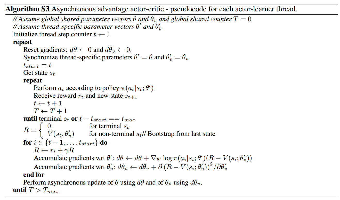
A3C is basically a bunch of A2C agents with a gradient reduction server. A3C(A2C) agents will interact with their environment simulators, train their local actors and critics, then push gradients to the gradient reduction server, the gradient reduction server will apply reduced gradients to its internal models (managed actor and critic network), then push the updated parameters to a key-value server. Agents will be able to pull the newest parameters and continue updating.

All A3C agents are fully asynchronous, gradient pushing & parameter pulling are asynchronous as well.

We will use the “CartPole-v0” environment from OpenAI Gym as an example, the actor network and critic network are as follows:

class Actor(nn.Module):
    def __init__(self, state_dim, action_num):
        super(Actor, self).__init__()

        self.fc1 = nn.Linear(state_dim, 16)
        self.fc2 = nn.Linear(16, 16)
        self.fc3 = nn.Linear(16, action_num)

    def forward(self, state, action=None):
        a = t.relu(self.fc1(state))
        a = t.relu(self.fc2(a))
        probs = t.softmax(self.fc3(a), dim=1)
        dist = Categorical(probs=probs)
        act = (action
               if action is not None
               else dist.sample())
        act_entropy = dist.entropy()
        act_log_prob = dist.log_prob(act.flatten())
        return act, act_log_prob, act_entropy


class Critic(nn.Module):
    def __init__(self, state_dim):
        super(Critic, self).__init__()

        self.fc1 = nn.Linear(state_dim, 16)
        self.fc2 = nn.Linear(16, 16)
        self.fc3 = nn.Linear(16, 1)

    def forward(self, state):
        v = t.relu(self.fc1(state))
        v = t.relu(self.fc2(v))
        v = self.fc3(v)
        return v

In order to initialize the A3C framework, we need to first initialize the distributed world:

# initlize distributed world first
_world = World(world_size=3, rank=rank,
               name=str(rank), rpc_timeout=20)

then provide a PushPullGradServer to it, Machin provides some helpful utility functions to aid inexperienced users initialize the distributed environment easily:

from machin.frame.helpers.servers import grad_server_helper
servers = grad_server_helper(
    [lambda: Actor(observe_dim, action_num),
     lambda: Critic(observe_dim)],
    learning_rate=5e-3
)

Note all helpers from machin.frame.helpers.servers requires all processes in the distributed world to enter.

Finally we can compose the complete setup of A3C:

# initlize distributed world first
_world = World(world_size=3, rank=rank,
               name=str(rank), rpc_timeout=20)

actor = Actor(observe_dim, action_num)
critic = Critic(observe_dim)

# in all test scenarios, all processes will be used as reducers
servers = grad_server_helper(
    [lambda: Actor(observe_dim, action_num),
     lambda: Critic(observe_dim)],
    learning_rate=5e-3
)
a3c = A3C(actor, critic,
          nn.MSELoss(reduction='sum'),
          servers)

And start training, just as the A2C algorithm:

# manually control syncing to improve performance
a3c.set_sync(False)

# begin training
episode, step, reward_fulfilled = 0, 0, 0
smoothed_total_reward = 0
terminal = False

while episode < max_episodes:
    episode += 1
    total_reward = 0
    terminal = False
    step = 0

    state = t.tensor(env.reset(), dtype=t.float32).view(1, observe_dim)

    # manually pull the newest parameters
    a3c.manual_sync()
    tmp_observations = []
    while not terminal and step <= max_steps:
        step += 1
        with t.no_grad():
            old_state = state
            # agent model inference
            action = a3c.act({"state": old_state})[0]
            state, reward, terminal, _ = env.step(action.item())
            state = t.tensor(state, dtype=t.float32).view(1, observe_dim)
            total_reward += reward

            tmp_observations.append({
                "state": {"state": old_state},
                "action": {"action": action},
                "next_state": {"state": state},
                "reward": reward,
                "terminal": terminal or step == max_steps
            })

    # update
    a3c.store_episode(tmp_observations)
    a3c.update()

    # show reward
    smoothed_total_reward = (smoothed_total_reward * 0.9 +
                             total_reward * 0.1)
    logger.info("Process {} Episode {} total reward={:.2f}"
                .format(rank, episode, smoothed_total_reward))

    if smoothed_total_reward > solved_reward:
        reward_fulfilled += 1
        if reward_fulfilled >= solved_repeat:
            logger.info("Environment solved!")
            # will cause torch RPC to complain
            # since other processes may have not finished yet.
            # just for demonstration.
            exit(0)
    else:
        reward_fulfilled = 0

A3C agents should will be successfully trained within about 1500 episodes, they converge much slower than A2C agents:

[2020-07-31 00:21:37,690] <INFO>:default_logger:Process 1 Episode 1346 total reward=184.91
[2020-07-31 00:21:37,723] <INFO>:default_logger:Process 0 Episode 1366 total reward=171.22
[2020-07-31 00:21:37,813] <INFO>:default_logger:Process 2 Episode 1345 total reward=190.73
[2020-07-31 00:21:37,903] <INFO>:default_logger:Process 1 Episode 1347 total reward=186.41
[2020-07-31 00:21:37,928] <INFO>:default_logger:Process 0 Episode 1367 total reward=174.10
[2020-07-31 00:21:38,000] <INFO>:default_logger:Process 2 Episode 1346 total reward=191.66
[2020-07-31 00:21:38,000] <INFO>:default_logger:Environment solved!

DQNApex and DDPGApex

Full code: DQNApex code

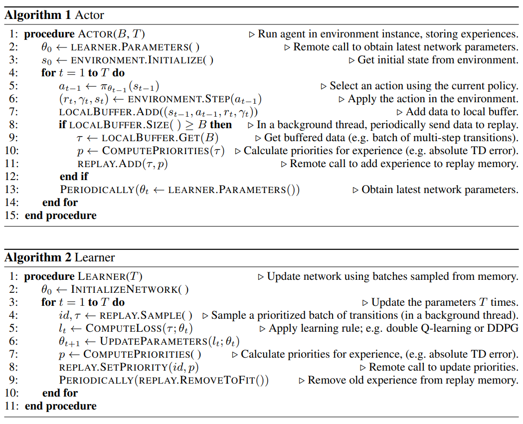
DQNApex and DDPGApex are actually based on the same architecture, therefore in this section, we are going to take DQNApex as an example, its distributed architecture could be described in the following graph:

Fig. 7 DQNApex architecture

And the pseudo code in essay:

Fig. 8 DQN-Apex pesudo code

The Apex architecture decouples the sampling and updating process with the prioritized replay buffer. There could be several implementations, such as:

1. using a central replay buffer on a single process

2. using a distributed buffer, with a central stopping signal.

3. using a distributed buffer, each buffer with a separate lock.

Machin choose the third implementation because it is most efficient:

#1 is slow because each appending requires a RPC process to update the global weight tree, and it also doesn’t scale when the number of workers(samplers) grows too large, such as 100+ workers.

The central lock used in #2 is meant to protect the importance sampling-updating process, so each buffer maintains a local weight tree, during sampling, the learner will signal “STOP” to all workers, and signal “START” to all workers when importance weight update is completed, however, this design does not truly decouples learning and sampling, therefore most of the time workers are just hanging and wait for the learner to complete updaing.

#3 design is the best, because each append operation is completely local (only needs to acquire a local lock), and global sampling is complete decoupled from local appending (because lock are immediately released after returning sampled data, and not till update complete) as show in figure Fig. 7.

However, it could be very tricky to implement this process, because appending is still happening after sampling and before the learner finishes updating importance sampling weights (is-weights), therefore Machin uses a taint table, which is essentially a table full of auto increment counters, each counter maps to an entry slot in the lower ring buffer, and is incremented if the entry has been replaced with new entries. This replacement should will not be very often if the buffer has enough space, (100000+), therefore guarantee the correctness of importance weight update.

There is one thing to note, it could be indefinitely long for learner to calculate the virtual global weight sum tree using the root node of all local weight sum trees as leaves, therefore at the time of sampling, the used weight sum of local trees is already outdated, and sampling probability of each tree should have changed. However, if the size of each local buffer is large enough, then the ratio of difference between the old collected local weight sums and current weight sums should be acceptable.

Now that we know how the Apex framework is designed, we may try an example. We will use the “CartPole-v0” environment from OpenAI Gym as an example, the Q networks is as follows:

class QNet(nn.Module):
    def __init__(self, state_dim, action_num):
        super(QNet, self).__init__()

        self.fc1 = nn.Linear(state_dim, 16)
        self.fc2 = nn.Linear(16, 16)
        self.fc3 = nn.Linear(16, action_num)

    def forward(self, some_state):
        a = t.relu(self.fc1(some_state))
        a = t.relu(self.fc2(a))
        return self.fc3(a)

Because apex frameworks relies on the DistributedPrioritizedBuffer, the learner needs to know the position and service name of each local buffer, as show in figure Fig. 7, in order to initialize the Apex framework, we need to provide a RPC process group, where all learner(s) and workers will live on:

apex_group = world.create_rpc_group("apex", ["0", "1", "2"])

And we will also provide a model server on which learner(s) will store the newest parameters and workers will pull the newest parameters from the server. This kind of parameter server is different from the PushPullGradServer used above, and we will name it as PushPullModelServer, Currently, each PushPullModelServer only manages one model per server instance, and since there is only one model needs to be shared in DQN (the online Q network), we only need one model server instance:

servers = model_server_helper(model_num=1)
dqn_apex = DQNApex(q_net, q_net_t,
                   t.optim.Adam,
                   nn.MSELoss(reduction='sum'),
                   apex_group,
                   (servers[0],),
                   replay_device=c.device,
                   replay_size=c.replay_size)

The tasks of learner(s) and workers are quite a bit different, since learner(s) only needs to update their internal models repeatedly, using samples from workers’ buffers, and workers only need to do update-sample-update-sample…, they will run different branches in the main program.

Maybe you want to ask, why are we using learner(s), isn’t the original essay stating that there is only one learner and multiple workers? The answer is: Machin supports using DistributedDataParallel (DataParallel is also supported) from PyTorch inside DQNApex, so that you may distribute the updating task across multiple learner processes, if your models is way too large to be computed by a single process. It is not sensible to using this technique with small models, but for pure demonstration purpose, we will use it here:

if rank in (2, 3):
    # learner_group.group is the wrapped torch.distributed.ProcessGroup
    learner_group = world.create_collective_group(ranks=[2, 3])

    # wrap the model with DistributedDataParallel
    # if current process is learner process 2 or 3
    q_net = DistributedDataParallel(module=QNet(observe_dim, action_num),
                                    process_group=learner_group.group)
    q_net_t = DistributedDataParallel(module=QNet(observe_dim, action_num),
                                      process_group=learner_group.group)
else:
    q_net = QNet(observe_dim, action_num)
    q_net_t = QNet(observe_dim, action_num)

# we may use a smaller batch size to train if we are using
# DistributedDataParallel
dqn_apex = DQNApex(q_net, q_net_t,
                   t.optim.Adam,
                   nn.MSELoss(reduction='sum'),
                   apex_group,
                   (servers[0],),
                   batch_size=50)

The main part of the training process is as follows:

# synchronize all processes in the group, make sure
# distributed buffer has been created on all processes
# in apex_group
apex_group.barrier()

# manually control syncing to improve performance
dqn_apex.set_sync(False)
if rank in (0, 1):
    # Process 0 and 1 are workers(samplers)
    # begin training
    episode, step, reward_fulfilled = 0, 0, 0
    smoothed_total_reward = 0

    while episode < max_episodes:
        # sleep to wait for learners keep up
        sleep(0.1)
        episode += 1
        total_reward = 0
        terminal = False
        step = 0

        state = t.tensor(env.reset(), dtype=t.float32).view(1, observe_dim)

        # manually pull the newest parameters
        dqn_apex.manual_sync()
        while not terminal and step <= max_steps:
            step += 1
            with t.no_grad():
                old_state = state
                # agent model inference
                action = dqn_apex.act_discrete_with_noise(
                    {"state": old_state}
                )
                state, reward, terminal, _ = env.step(action.item())
                state = t.tensor(state, dtype=t.float32)\
                    .view(1, observe_dim)
                total_reward += reward

                dqn_apex.store_transition({
                    "state": {"state": old_state},
                    "action": {"action": action},
                    "next_state": {"state": state},
                    "reward": reward,
                    "terminal": terminal or step == max_steps
                })

        smoothed_total_reward = (smoothed_total_reward * 0.9 +
                                 total_reward * 0.1)
        logger.info("Process {} Episode {} total reward={:.2f}"
                    .format(rank, episode, smoothed_total_reward))

        if smoothed_total_reward > solved_reward:
            reward_fulfilled += 1
            if reward_fulfilled >= solved_repeat:
                logger.info("Environment solved!")

                # will cause torch RPC to complain
                # since other processes may have not finished yet.
                # just for demonstration.
                exit(0)
        else:
            reward_fulfilled = 0

elif rank in (2, 3):
    # wait for enough samples
    while dqn_apex.replay_buffer.all_size() < 500:
        sleep(0.1)
    while True:
        dqn_apex.update()

Result:

[2020-08-01 12:51:04,323] <INFO>:default_logger:Process 1 Episode 756 total reward=192.42
[2020-08-01 12:51:04,335] <INFO>:default_logger:Process 0 Episode 738 total reward=187.58
[2020-08-01 12:51:04,557] <INFO>:default_logger:Process 1 Episode 757 total reward=193.17
[2020-08-01 12:51:04,603] <INFO>:default_logger:Process 0 Episode 739 total reward=188.72
[2020-08-01 12:51:04,789] <INFO>:default_logger:Process 1 Episode 758 total reward=193.86
[2020-08-01 12:51:04,789] <INFO>:default_logger:Environment solved!

IMPALA

Full code: IMPALA code

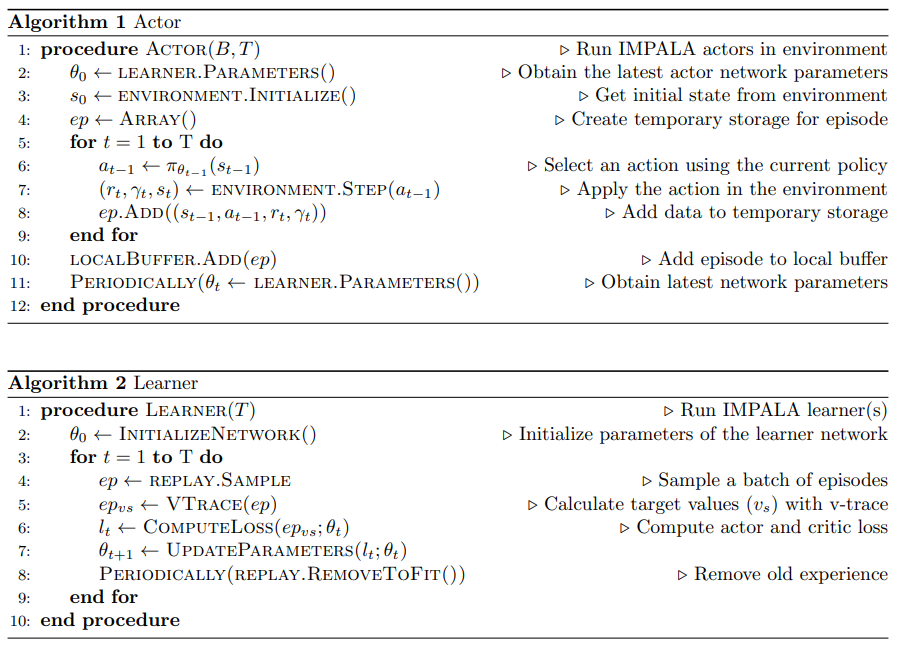
The IMPALA algorithm has the same parallel architecture as DQNApex and DDPGApex do, the only difference is that the internal distributed buffer it is using is a simple distributed buffer, with no distributed prioritized tree:

Fig. 9 Impala architecture

The pseudo code of the IMPALA algorithm is as follows:

Fig. 10 Impala pesudo code

where the \(VTrace\) function is defined as:

\[ \begin{align}\begin{aligned}& v_s = V(X_s) + \sum_{t=s}^{s+n-1} \gamma^{t-s} (\prod_{i=s}^{t-1} c_i) \delta_t V\\& \delta_t V = \rho_t(r_t + \gamma V(x_{t+1}) - V(x_t))\\& \rho_t = min(\rho_{max}, \frac{\pi(a_t | x_t)}{\mu (a_t | x_t)})\\& c_i = min(c_{max}, \frac{\pi(a_i | x_i)}{\mu (a_i | x_i)})\end{aligned}\end{align} \]

In order to initialize the IMPALA framework, we need to pass two accessors to two individual PushPullModelServer to the framework, and take note that IMPALA does not support storing a single step**, since v-trace calculation requires sampling complete episodes, all transition objects in the IMPALA buffer are episodes rather than steps, therefore the used batch_size is set to 2, which is much smaller then 50 used in DQNApex:

if rank in (2, 3):
    # learner_group.group is the wrapped torch.distributed.ProcessGroup
    learner_group = world.create_collective_group(ranks=[2, 3])

    # wrap the model with DistributedDataParallel
    # if current process is learner process 2 or 3
    actor = DistributedDataParallel(module=Actor(observe_dim, action_num),
                                    process_group=learner_group.group)
    critic = DistributedDataParallel(module=Critic(observe_dim),
                                     process_group=learner_group.group)
else:
    actor = Actor(observe_dim, action_num)
    critic = Critic(observe_dim)

# we may use a smaller batch size to train if we are using
# DistributedDataParallel

# note: since the impala framework is storing a whole
# episode as a single sample, we should wait for a smaller number
impala = IMPALA(actor, critic,
                t.optim.Adam,
                nn.MSELoss(reduction='sum'),
                impala_group,
                servers,
                batch_size=2)

The main part of the training process is almost the same as that of DQNApex:

# synchronize all processes in the group, make sure
# distributed buffer has been created on all processes in apex_group
impala_group.barrier()

# manually control syncing to improve performance
impala.set_sync(False)
if rank in (0, 1):
    # Process 0 and 1 are workers(samplers)
    # begin training
    episode, step, reward_fulfilled = 0, 0, 0
    smoothed_total_reward = 0

    while episode < max_episodes:
        # sleep to wait for learners keep up
        sleep(0.1)
        episode += 1
        total_reward = 0
        terminal = False
        step = 0

        state = t.tensor(env.reset(), dtype=t.float32).view(1, observe_dim)

        # manually pull the newest parameters
        impala.manual_sync()
        tmp_observations = []
        while not terminal and step <= max_steps:
            step += 1
            with t.no_grad():
                old_state = state
                # agent model inference
                action, action_log_prob, *_ = \
                    impala.act({"state": old_state})
                state, reward, terminal, _ = env.step(action.item())
                state = t.tensor(state, dtype=t.float32) \
                    .view(1, observe_dim)
                total_reward += reward

                tmp_observations.append({
                    "state": {"state": old_state},
                    "action": {"action": action},
                    "next_state": {"state": state},
                    "reward": reward,
                    "action_log_prob": action_log_prob.item(),
                    "terminal": terminal or step == max_steps
                })

        impala.store_episode(tmp_observations)
        smoothed_total_reward = (smoothed_total_reward * 0.9 +
                                 total_reward * 0.1)
        logger.info("Process {} Episode {} total reward={:.2f}"
                    .format(rank, episode, smoothed_total_reward))

        if smoothed_total_reward > solved_reward:
            reward_fulfilled += 1
            if reward_fulfilled >= solved_repeat:
                logger.info("Environment solved!")

                # will cause torch RPC to complain
                # since other processes may have not finished yet.
                # just for demonstration.
                exit(0)
        else:
            reward_fulfilled = 0

elif rank in (2, 3):
    # wait for enough samples
    # note: since the impala framework is storing a whole
    # episode as a single sample, we should wait for a smaller number
    while impala.replay_buffer.all_size() < 5:
        sleep(0.1)
    while True:
        impala.update()

IMPALA converges very fast, usually within 150 episodes:

[2020-08-01 23:25:34,861] <INFO>:default_logger:Process 1 Episode 72 total reward=185.32
[2020-08-01 23:25:35,057] <INFO>:default_logger:Process 1 Episode 73 total reward=186.79
[2020-08-01 23:25:35,060] <INFO>:default_logger:Process 0 Episode 70 total reward=193.28
[2020-08-01 23:25:35,257] <INFO>:default_logger:Process 1 Episode 74 total reward=188.11
[2020-08-01 23:25:35,261] <INFO>:default_logger:Process 0 Episode 71 total reward=193.95
[2020-08-01 23:25:35,261] <INFO>:default_logger:Environment solved!